What, then, are the parameters of the normal distribution? An idealized, normal distribution is fully determined given two quantities: its midpoint and its width. As already mentioned, normal distributions are special, because their symmetry and short tails means that it has a “central tendency” that can be used as a model to predict its value and summarize a dataset. When the distribution is skewed, it becomes useful to distinguish between different measures of central tendency (mode, median and mean), but for a bell-shaped symmetrical one, these are the same, and coincide with the mid-point. However, because empirically derived distributions are never perfect, the arithmetic mean, which takes the most information into account, is the one used, and therefore the mid-point population parameter is the mean, even though it equals the others.
In the normal distribution the mode, the median and the mean are the same, but for approximations the mean is usually used, because it takes the most information into account. If the median is a fulcrum that balances the number of values on either side, the mean balances the number of total "value-units" on either side.
The mean, effectively, is like the fulcrum of a balanced pair of scales poised at the center of all deviations from itself. It is defined as the point where deviations from it sum to zero. Its width, the average deviation, is called “standard deviation”. The wider the distribution, the poorer the mean will be as a predictor, and the more noise in the data. The intuitive explanation for its formula leaves it slightly under-determined – it is motivated by the mathematical equation of the normal distribution – but is shown below.
Standard deviation is the width-parameter of the normal distribution and can be understood as "average deviation", but it is not strictly a mean deviation, since its formula gives disproportionate emphasis to large deviations.
Given a population that is known to be normal, statisticians can use the mean and the standard deviation to calculate a density function that associates a particular value-range with a probability (a single point-value has an infinitesimally small probability, so we can only consider intervals). Because regardless of the parameters, the same location of a range relative the mean (expressed in terms of standard deviations – a length unit, remember) has the same probability, it makes sense to re-express a certain value in terms of “distance from the mean” for a standard distribution. It is the equivalent of two tradesmen translating the value of their goods to a shared currency, and is called z-scores.
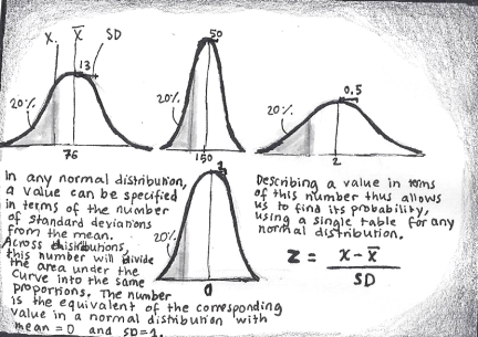
Standard (z) scores allow us to associate the range below/above a value on any normal distribution with a probability via a single table, by expressing them in terms of standard deviations from the mean.
Now recall that the Central Limit Theorem implies that large and unbiased samples will resemble the population from which it comes. The probability that any sample will deviate greatly from the population is low. Now imagine a weirdly distributed population, of known mean and SD, real or just a theoretical phantom, and, for a certain sample size, consider the space of all possible samples (i.e. subsets) that could be drawn from it. Take the mean of all those samples, erect a histogram, and call this the “sample distribution of the mean”. You may regard it as a population in its own right. Because of the central limit theorem (some averages are more common than others), this distribution will be more bell-shaped than the original distribution. The bigger sample size, the smoother it will be, and the better any theoretically based estimate will be.
For reasons that are intuitively clear, the population of the means of all possible samples drawn from a population distribution will have the same mean as itself. This means that there is a high likelihood that the samples you draw will have statistics that are similar to the parameters. Therefore, if you have your sample and know the population parameters, you may estimate how likely it is that the sample is indeed drawn from this population. If your sample mean has a score far to the right of the mean, the conditional probability P(score far away| score from population) is low.
Now suppose instead that the population distribution is unknown. Usually, your sample is the only information you have. Again, our goal is to construct a sample distribution of the mean to gauge where our sample falls on it. To do this, we need to know its width, that is, how much samples are expected to vary, in other words, its standard deviation of the sample means. We know that:
- For a large sample size, there will be less variability (since noise will be cancelled out, causing means to cluster tightly).
- For a large population SD, there will be more variability (since how much it is expected to vary depends on how much it actually varies). As said, the population SD is not available, so we have to base it on sample SD instead.
This calls for a mathematical formula with the sample SD as numerator (so that big SD causes a bigger value) and sample size as denominator (so that big N means a smaller value), and it goes by the name “Standard error of the mean” (which has the added quirk that the square root is taken from the denominator, because of the mathematics of the normal distribution).
To find how well parameter values predict a certain sample we need to calculate the equivalent of the z-score. However, this time, since our evidential support is so weak (we, for example, use sample mean to estimate population mean), modelling the sample distribution of the mean as a normal distribution would give us overconfidence in our estimates. We need a higher burden of proof. For this purpose, statisticians have come up with a distribution that has fatter tails (implying a larger z* critical value), which, cleverly, approaches the normal distribution for large sample sizes.
Thus, we have a way for estimating the conditional P(data|hypothesis) in a way that depends on sample size. It is from this point onwards that the different statistical procedures diverge in their prescriptions.